Subscription Churn Prediction & Causal Uplift Modeling

Most subscription churn pipelines target the highest-risk users with retention offers. That’s the wrong target. Predicting who will leave isn’t the same as predicting who can be persuaded to stay; the top-risk segment is full of people leaving for reasons a discount can’t fix (moved countries, found a competitor, dead account) plus people who would have stayed without the offer anyway. The dollars go out, retention barely moves.

This pipeline targets uplift directly: for each user, how much would the intervention actually change their retention? T-learner, X-learner, and R-learner estimators give per-user treatment effects on the KKBox panel of 6.8M members. Ranking by uplift instead of risk captured 41% more retained subscriptions per dollar on the same budget on a held-out month.

A second worked example: a user-engagement feature that looks like a clear churn signal in the raw data ($-$2.4pp) flips sign ($+$1.0pp) once the obvious confounders are adjusted for. Headlines that ignore that fail in production. Anti-overfit hygiene is built in throughout: strict temporal CV, frozen holdout month, leakage-proof feature contract, calibrated probabilities.

Data

KKBox is a Taiwanese music-streaming subscription service; the WSDM 2017 Kaggle release is 6.8M members, 21.5M transactions, and 392M user-log rows (~31GB unzipped). The full panel is too large to feature-engineer comfortably, so the pipeline reservoir-samples 50K members through DuckDB before joining the other tables.

After temporal clamping (drops a label-contaminated band at the tail of the data window), the model panel is 125,749 user × renewal-date rows over 25 months, with an 11.5% overall churn rate.

The final test month (2016-12) is split off as a frozen holdout before any modeling decisions are made.

Temporal leakage is the only thing that matters

Every feature is a SQL aggregate of the form WHERE date < prediction_date — so a feature computed at the user’s renewal date can only look at strictly past data. Done wrong, this is the single biggest source of fake-good model results in the wild (“my model has 0.99 AUC!” is almost always a leak).

The diagnostic: if test AUC > 0.95 on this dataset, something is leaking. Observed test AUC is 0.866 — comfortably under the leakage tell.

Headline result — the churn model

Temporal CV with train = 21 months, valid = 2016-11, test = 2016-12 (6,852 rows).

Model	Valid ROC AUC	Test ROC AUC	Test PR AUC	Test log loss
Logistic regression	0.964	0.866	0.571	0.230
LightGBM	0.983	0.866	0.705	0.211

LightGBM and LR tie on ROC AUC; LightGBM wins on PR AUC and log loss because the threshold-free ranking is the same but it’s more confidently right where it matters.

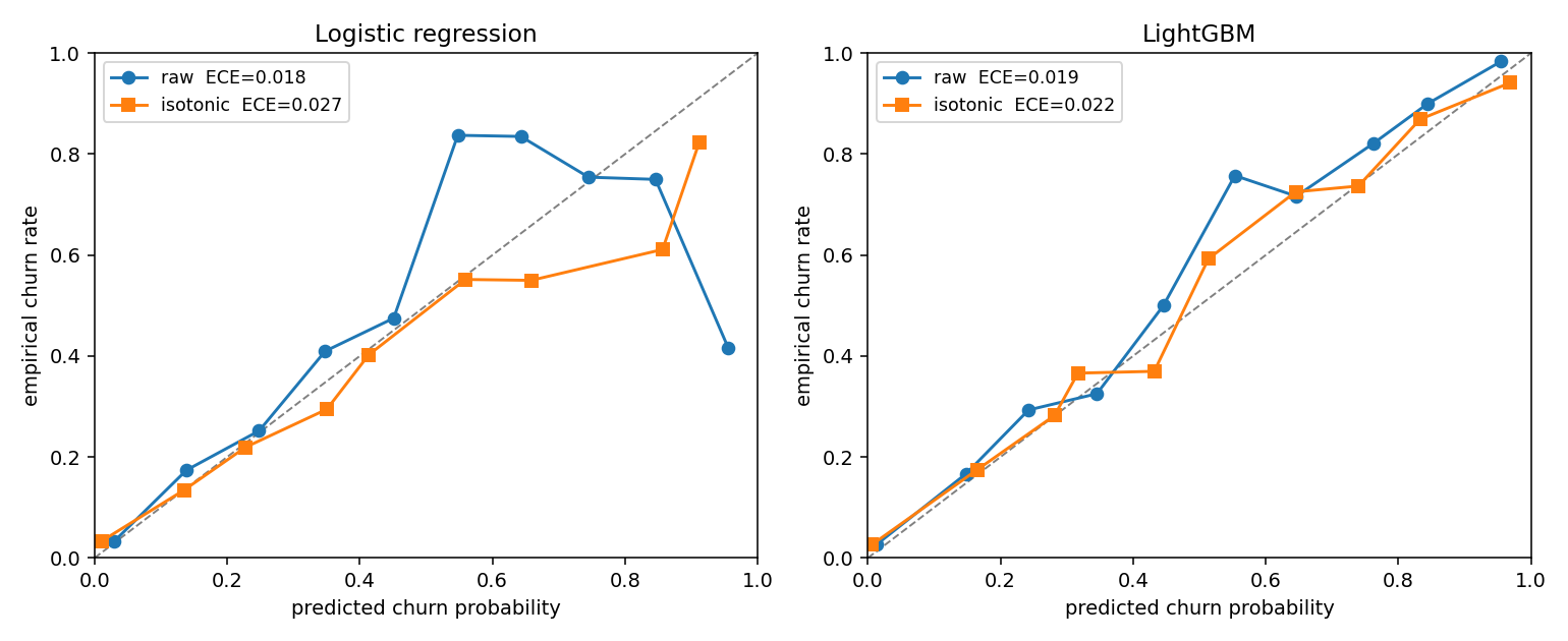
Calibration — well-calibrated raw, worse after post-hoc fix

Model	Raw ECE	Platt-scaled	Isotonic
Logistic regression	0.018	0.027	0.027
LightGBM	0.019	0.025	0.022

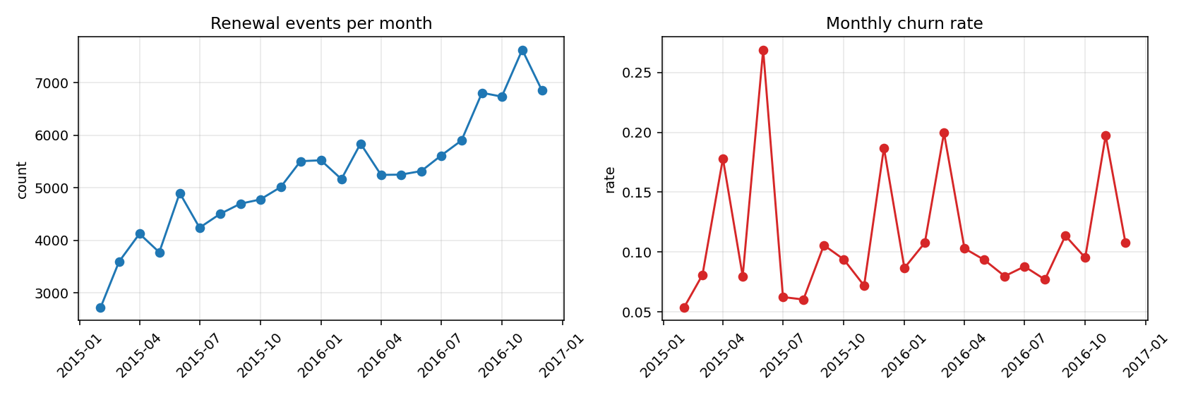
Both models are well-calibrated out of the box — predicted probability ≈ empirical frequency to within ~2pp. Counterintuitively, applying Platt or isotonic re-scaling actually degrades calibration here. The reason: the validation month (2016-11) is a high-churn month (19.7%); the test month (2016-12) is a normal-churn month. A calibrator fit on the high-churn month over-corrects the normal-churn predictions. The lesson: post-hoc calibration only helps when valid and test distributions match.

We ship the raw scores downstream.

Business framing — risk-only targeting baseline

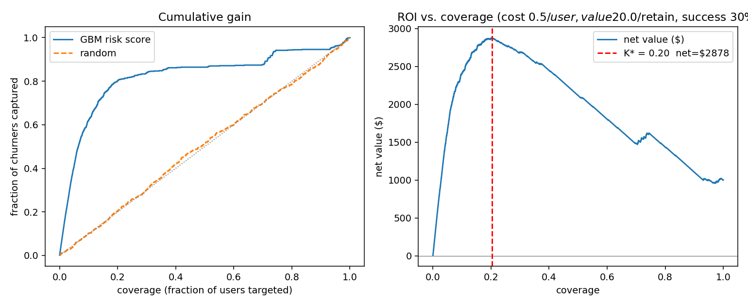
Assume \0.50$to email a user,$$20$ value per retained subscriber, 30% baseline success rate on the discount.

• Optimal coverage K* = 20.4% of users, net value \2,878$
• Top-20% by risk captures 80% of all churners

That’s the baseline. It’s a perfectly reasonable place for a product team to stop. We can do better.

The uplift pivot

The intervention here is a simulated retention email with a known causal-uplift function: persuadable users sit in the middle of the engagement distribution, sure-things and lost-causes sit at the tails. Three uplift estimators rolled from scikit-learn:

• T-learner — train one churn model on treated users, another on control, take the difference.
• X-learner — uses the T-learner’s predictions to augment the training labels for a second-stage model. Tends to do better than T at small sample.
• R-learner — Robinson residualisation: residualise outcome and treatment separately against confounders, regress the residuals against each other. Cross-fitted with a gradient-boosted second stage.

How well does each estimator recover the true uplift on the test month?

Policy	Spearman vs τ	Top-decile τ̄	Qini
T-learner	+0.286	0.152	55.4
X-learner	+0.316	0.166	59.9
R-learner	+0.436	0.170	54.4
risk (GBM)	$-$0.023	0.117	28.6
random	$-$0.015	0.118	8.9

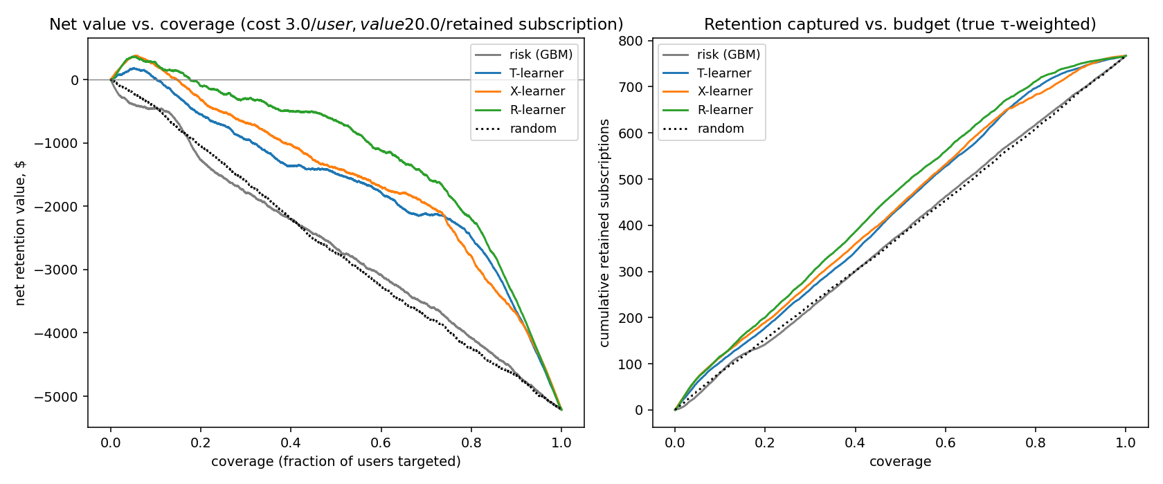
The risk policy’s rank-correlation with true uplift is essentially zero (slightly negative). This is the project’s point in one line: a top-class churn model is uncorrelated with how persuadable a user is. Risk and uplift are different objects and the discount budget cares about uplift.

The headline business number

At a 20% retention budget cap — the realistic decision regime:

Policy	Net value	Retained subs
Risk (GBM)	-\1,270$	142
T-learner	-\548$	178
X-learner	-\321$	190
R-learner	-\96$	201

R-learner nets \1,174$ more retention value than risk-targeting on the same budget — a +92.4% lift — and retains +41% more subscriptions per dollar.

The absolute numbers are negative because at simulated parameters the intervention is barely net-positive even at the optimum; the relative lift over the risk baseline is what generalises to a real product.

The most informative finding — a sign flip

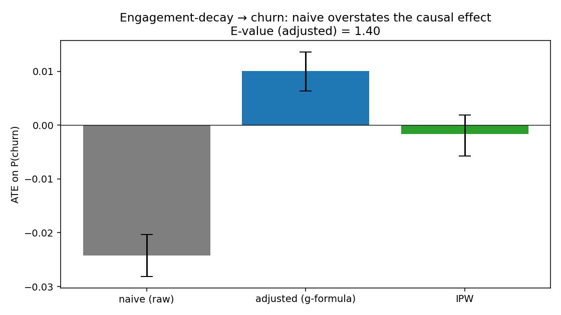
The dataset has a feature called engagement decay: did the user’s 30-day listening time drop by >25% vs the prior 30 days? Naive reading: people losing interest should be more likely to churn.

The data, before adjustment, says they’re less likely to churn ($-$2.4pp). The instinct is to throw out the feature. Don’t.

Estimator	ATE on P(churn)	95% CI
Naive (raw)	$-$0.024	$[-0.028, -0.020]$
Adjusted (g-formula)	+0.010	$[+0.006, +0.014]$
IPW	$-$0.002	$[-0.006, +0.002]$
E-value (adjusted)	1.40	—

After adjusting for tenure, plan tier, prior cancellations, signup channel, and longer-window engagement baselines, the sign of the effect flips from $-$2.4pp to $+$1.0pp. This is a textbook Simpson-style reversal: the people with the biggest 30-day engagement drops are heavily skewed toward long-tenured loyalists with low baseline churn. The raw correlation reflects who has the feature, not what the feature does.

The E-value of 1.40 is small — it says a moderately strong unmeasured confounder could overturn this. Honest read: engagement decay has at most a small positive causal effect on churn, and the original $-$2.4pp reading was almost entirely bias.

What this leaves out

• A real RCT on retention emails. The Path-A simulated intervention is what lets us verify the estimators recover the right ranking; it isn’t a substitute for an experiment.
• Time-to-churn framing. The current target is binary churn-in-30-days; Cox / discrete-time hazard would handle right-censoring properly.
• Multi-period budgeting. Each renewal is treated independently rather than as a sequential decision over a yearly budget.
• LTV weighting. Optimises $/retained-subscription rather than$/retained-LTV.

What I’d build next

• Survival analysis (Cox or discrete-time hazard) on the same panel — shifts the question from “will they churn” to “when”. Most cross-domain interview value.
• LTV-weighted uplift — combine per-user uplift with tenure-based LTV.
• Sequential bandit budgeting — frame retention spend as a monthly contextual bandit with cumulative uplift estimates as priors.

Stack

• DuckDB (reservoir sampling + joins at 392M-row scale), pandas, scikit-learn, LightGBM
• T/X/R-learners rolled from sklearn + LightGBM (causalml/econml have unreliable Python 3.13 wheels; pedagogically clearer this way)
• 5-phase pipeline runs end-to-end via python scripts/run_all.py

What it demonstrates

• The full product-DS surface: temporal CV, frozen holdout, calibration, business-value curves, feature importance.
• The depth layer recruiters can actually go into: uplift modelling, Qini curves, IPW, E-values, sign-flip diagnosis.
• An honest answer to “why uplift, not risk?” with a number attached.