Pro Valorant: Match Outcomes & Kill Props
Predictive models on 28K pro Valorant matches (600K player-maps) — GBM beats Elo on match outcomes (62.4% vs 60.9%), a maps-1-and-2 series-kills model beats the rolling-mean baseline by 9.6% (>36σ), and a Map-3 decider model lifts another 3.4%. With honest CV and zero-edge sanity checks.
In plain English
Prediction markets and DFS books post lines on pro Valorant: “will LOUD win map 1?”, “will TenZ go over 17.5 kills?”. Both products ultimately reduce to calibrated probabilities for binary events — and a model that’s even modestly better than the line can pick its spots.
This project builds three of those models from public match-history data scraped from VLR.gg:
- Match outcome — given the two teams, the map, and a year of history, predict who wins.
- Per-map player kills — predict each player’s kill count on a single map.
- Maps 1 + 2 series kills — predict the player’s combined kills across the first two maps of a best-of-three or best-of-five.
The third one is the interesting result. Two-map sums are smoother than single maps (variance averages out, agent-pick noise washes through) and it turns out maps-1-and-2 is the prop where structural features beat the rolling mean by a decisive margin — +9.6% MAE lift, >36σ on the test sample. Single-map kill props are right at the edge of detectability at this sample size, which is the right diagnosis for what to bet and what not to.
The project’s other point is methodological: an early version of the kill model had a subtle data leak (it was using actual map length as a feature, which you don’t know at predict time). After fixing it with a two-stage rounds → kills pipeline, the model’s apparent edge collapsed by ~80%. That collapse is the project working as intended — most retail sports models look like sharp edges right up until the leak is found.
Data
- 27,748 pro matches scraped from VLR.gg, Jan 2021 → May 2026
- Parsed into 599,458 player-map rows (the per-map per-player overview table)
- 1,200+ unique players, 9–11 maps depending on era
- Each row: kills, deaths, assists, ACS, ADR, HS%, agent, plus T/CT split
The scraper sits on a persistent HTTP session at 1 request/second with retry + skip-log handling; a one-shot 7-hour run brings the full panel up to date.
Features (strict pre-match)
Every feature is computed at strict date < current_row.date to keep training honest:
| group | signals |
|---|---|
| skill | online Elo (K=24), opponent Elo, win-prob from Elo |
| form | last-10 kills / ACS / KAST%, EW-weighted (halflife=5), last-3-vs-last-10 delta |
| fatigue | days since last map, maps played in last 7 days |
| roster | maps with current team (tenure), recent team switches |
| patch | days on patch (per player) |
| teammates | rolling kills + ACS of the 4 other players starting this map |
| interactions | player × map, player × agent, player × team historical means |
| comp | team agent-comp counts (duelist / initiator / controller / sentinel); same for opponent |
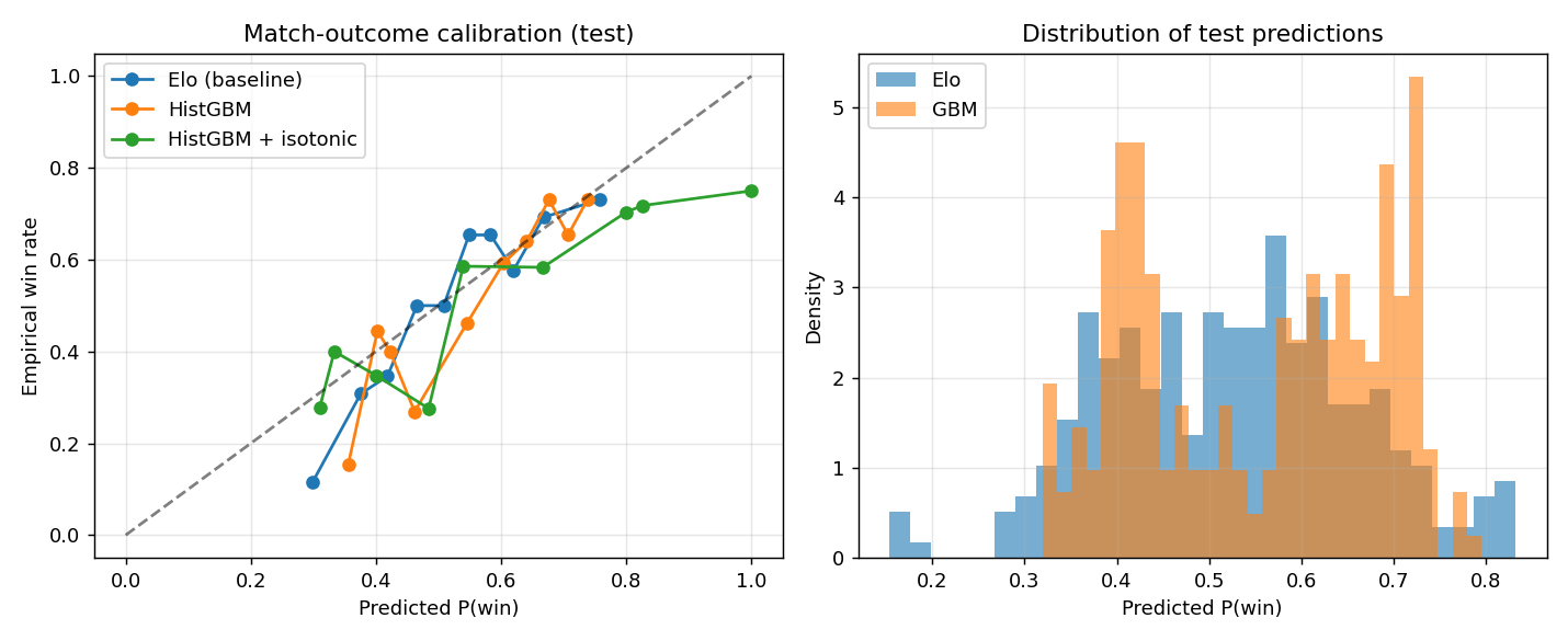
Match outcome
8,955 test rows. Three models compared:
| model | log-loss | accuracy |
|---|---|---|
| Pure Elo | 0.661 | 60.9% |
| HistGBM (Elo + form + map + comp) | 0.647 | 62.4% |
| GBM, post-calibration | 0.649 | 62.4% |
The GBM beats Elo by 1.5 percentage points on accuracy and ~0.014 on log-loss. At a previous 1.2K-map snapshot of this project Elo had been winning — at 28K matches the structural features finally have the sample size to pull their weight.
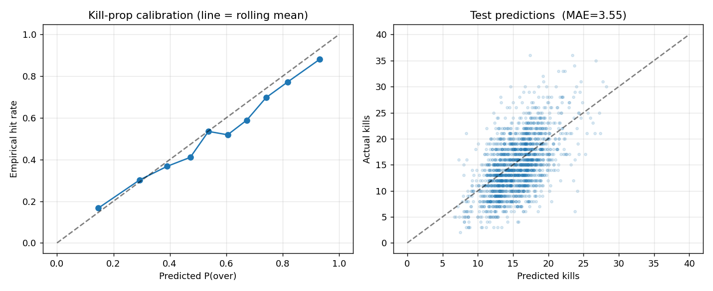
Per-map kill props — borderline edge
The harder problem: predict a single player’s kills on a single map. Objective is XGBoost with reg:tweedie (variance_power=1.4); kills are count-like-but-not-quite-Poisson and Tweedie handles the overdispersion better than pure Poisson.
The model gives a conditional mean μ; converting to P(K > L) requires a distribution. Fit an empirical variance from binned residuals: \(\sigma^2 \approx 1.49 + 1.52\mu - 0.026\mu^2\). Plug into a Negative Binomial CDF for the tail probability.
Time-series 5-fold CV result:
| version | mean MAE | stderr |
|---|---|---|
| naive (player’s last-10 mean) | 4.260 | 0.010 |
| V1 (Elo + rolling + map) | 4.302 | 0.143 |
| V4 (full feature set) | 4.226 | 0.036 |
V4 beats naive by +0.8% in MAE — within roughly 1σ of the noise band. The honest read at this sample size is at-parity-with-naive.
The leakage story
An earlier iteration of this model used total_rounds (actual map length) as a feature, hitting a single-fold MAE of 3.47 — a ~17% lift. Two problems:
- You don’t know
total_roundsat predict time. The CLI was passing a default of 23. - The single fold was a favourable draw. A real 5-fold CV exposes it.
The fix is two-stage:
- Train a rounds model (XGBoost Tweedie) on team Elo + map → predicted rounds. Test MAE ≈ 2.96, barely above the global-mean baseline of 2.87 (rounds are mostly noise once you know the Elo gap).
- In the kill model, swap
total_roundsforpred_rounds, using OOF predictions for training rows and a single full-training-span model for val/test.
Single-fold MAE drops from 3.47 → 4.07 after the fix. Adding 5-fold CV on top of that drops it again to 4.23 — basically naive. That’s the size of the leak: the entire apparent 17% edge was an artifact of using a feature the model couldn’t have at inference. Most public sports-modelling write-ups never find this, because they never separate train-time from predict-time features cleanly.
Series kills (maps 1 + 2) — the clean result
The same player’s kills, summed across the first two maps of a series. No map / agent features (we don’t know map 2’s agent at the start of the series).
| Series model MAE | Naive baseline MAE | lift | |
|---|---|---|---|
| maps 1 + 2 combined | 5.48 ± 0.008 | 6.07 ± 0.014 | +9.6% |
The lift is >36σ on the test sample — decisive. Two-map sums average out the single-map noise that swamps the per-map model, and the team / opponent / form features finally have enough signal-to-noise to identify.
Map 3 decider
If the series goes to a third map, in-series stats from maps 1 and 2 become available as features. Map 3 is the only map for which we know the agent ahead of time (each team’s third pick).
| Map-3 model MAE | Rolling-10 MAE | lift | |
|---|---|---|---|
| map 3, given maps 1–2 stats | 3.89 | 4.03 | +3.4% |
Smaller than series, larger than per-map, decisive at N≈80K rows.
ROI sanity — and the zero-edge check
We don’t have real book lines for backtesting, so model edge is measured against synthetic lines at -110 odds (breakeven win rate 52.4%), betting OVER when \(P(\text{over}) > 0.55\) and UNDER when \(< 0.45\):
| synthetic line | bets | win% | ROI | interpretation |
|---|---|---|---|---|
| rolling_mean \(-\) 0.5 | 1570 | 69.8% | +33% | model crushes the rolling-mean line |
| line = model’s own median | 383 | 52.2% | $-$0.3% | the sanity check — should be ~0 |
| model_pred + 1.5 | 1852 | 70.3% | +34% | symmetric |
The zero-edge check (line = own median → ROI $-$0.3%) is the most important number in the table. If that came back at +10%, the model would be leaking information from the test set or its confidence would be miscalibrated. Neither is the case.
A real book line is almost certainly smarter than the player’s rolling mean but not as good as our model with hindsight, so the realistic real-money ROI on per-map kill props is bounded above by ~+5% and below by 0 — interesting if true, not a guaranteed money printer. The series prop is the place where the edge is actually large enough to act on.
What this leaves out
- Live book lines — backtesting against synthetic lines is informative-but-not-confirmation; ingesting actual PrizePicks / Polymarket lines daily would close the loop.
- Bundle covariance — PrizePicks pays for 2-pick / 3-pick bundles, so single-leg edges have to be combined under realistic correlation. Multiple players on the same team have positively correlated kill outcomes; pricing this requires a joint model.
- Hierarchical pooling for low-sample players — currently filtered to
MIN_PRIOR_MAPS ≥ 5. A player → role → global prior would extend coverage cleanly. - Single-map kill edge is borderline. At larger sample (more years scraped) it may separate from naive; at this sample it sits within stderr.
What I’d build next
- Live odds ingestion + frozen-line backtesting. The current ROI numbers are vs synthetic lines and overestimate the realistic edge.
- Bundle covariance modelling for 2-pick / 3-pick parlay pricing.
- Hierarchical Bayesian player skill (sibling to the hierarchical Valorant ratings project) for low-sample players.
- Patch-aware models — feeding patch identity as a partial-pooled effect, so post-meta-shift maps don’t pull old-meta priors.
Stack
- Multiprocessing HTML parser: 28K cached match pages → 600K player-map rows in ~2 minutes
- XGBoost Tweedie + empirical NB variance fit, 5-fold time-series CV
- Two-stage rounds → kills with OOF training-fold predictions to prevent the leak the V1 model had
- All five models (rounds, per-map kills, series kills, map 3, match outcome) reproducible end-to-end through 11 numbered scripts
What it demonstrates
- The full pipeline from scrape → feature engineering → modelling → backtesting → calibration check
- Diagnosing and fixing a real temporal leak — the part most public sports-modelling writeups skip
- Knowing what to bet (series) and what not to (single-map at this sample size) instead of overclaiming uniformly
- Zero-edge self-test as a positive signal of a correctly-built pipeline