Hierarchical Bayesian Skill Rating for Pro Valorant
Hierarchical Bradley–Terry with map, region, and time pooling. On 86 held-out cross-regional matches, log loss 0.600 vs Elo’s 0.640 (95% CI [−0.019, +0.098]); ECE drops 0.092 → 0.060 and confident calls (≥70%) land at 78% empirical.
In plain English
Most rating systems used in competitive play (chess Elo, video-game ladder MMR) are essentially online point-trackers: you win, your number goes up; you lose, it goes down. They’re simple, well-understood, and they have a real weakness — they can’t say how certain they are about any particular team’s number, and they can’t share information across structural features of the game (which map you’re playing, which region you came up in, how much your roster has churned).
This project replaces the point-tracker with a hierarchical Bayesian model: every team gets a probability distribution over its skill, those distributions are anchored by regional priors that themselves get learned from the data, and per-team-per-map and time-drift effects fall out as natural extensions. On a held-out set of 86 cross-regional matches the model never trained on, the full hierarchy beats Elo by 0.040 log-loss (paired-bootstrap 95% CI [−0.019, +0.098]); calibration improves more cleanly (ECE 0.092 → 0.060). The improvement is suggestive but not strictly significant at this sample size — the natural way to nail it down is to extend the panel through Masters Tokyo and Champions LA, which would roughly triple the cross-regional signal.
Setup
Outcome. One row per map played. Predict P(team A wins the map). Map-level rather than match-level: ~3× the data and exposes map-specific structure that match-level outcomes hide.
Test design. Two complementary held-out evaluations:
- Chronological holdout — last 20% of dates (n=106, all VCT regional-league playoffs in late May 2023). The conventional time-series test.
- Cross-regional held-out (n=86) — every cross-regional match in the panel hidden from training, then predicted. The test the regional hierarchy is designed for.
Slice 1 is dense within-region late-season play; slice 2 is sparse cross-regional play between teams that don’t otherwise meet.
Data
VLR.gg match pages from 2022-09-01 through 2023-05-28, scraped and parsed into one row per map (reusing the scraper from the Patch 5.12 Chamber project). After region re-bucketing, partner-team filtering, and a min-5-appearances activity filter, the panel is 502 maps across 30 teams in three home regions (Americas, EMEA, Pacific).
| Train | Test | |
|---|---|---|
| Rows | 396 | 106 |
| Date range | 2022-09-01 – 2023-05-17 | 2023-05-18 – 2023-05-28 |
| Cross-regional | 86 | 0 |
| Tournament tiers | VCT regional + LOCK//IN + Champions 2022 | VCT regional playoffs only |
A note on the scraper. The upstream Chamber project’s region classifier had a bug — its Pacific-keyword list contained " sea" (intended for “SEA” = Southeast Asia) which silently matched "season" in event names like “Champions Tour 2023: Americas League — Regular Season Week 1”, mis-bucketing LOUD, NRG, and other Americas teams as Pacific. I re-derived region bucketing against league-name tokens (e.g. "americas league", "vct emea").
Phase 1 — Baselines
Win-rate baseline. P(A wins) = A’s pre-row win rate / (A’s + B’s), with a Beta(2.5, 2.5) prior so cold teams sit near 0.5.
Elo. Standard Elo over map outcomes. K-factor tuned by within-train chronological holdout — best K = 48 (grid 8–96). Higher than chess Elo (K~16); the panel is short enough that aggressive updating helps.
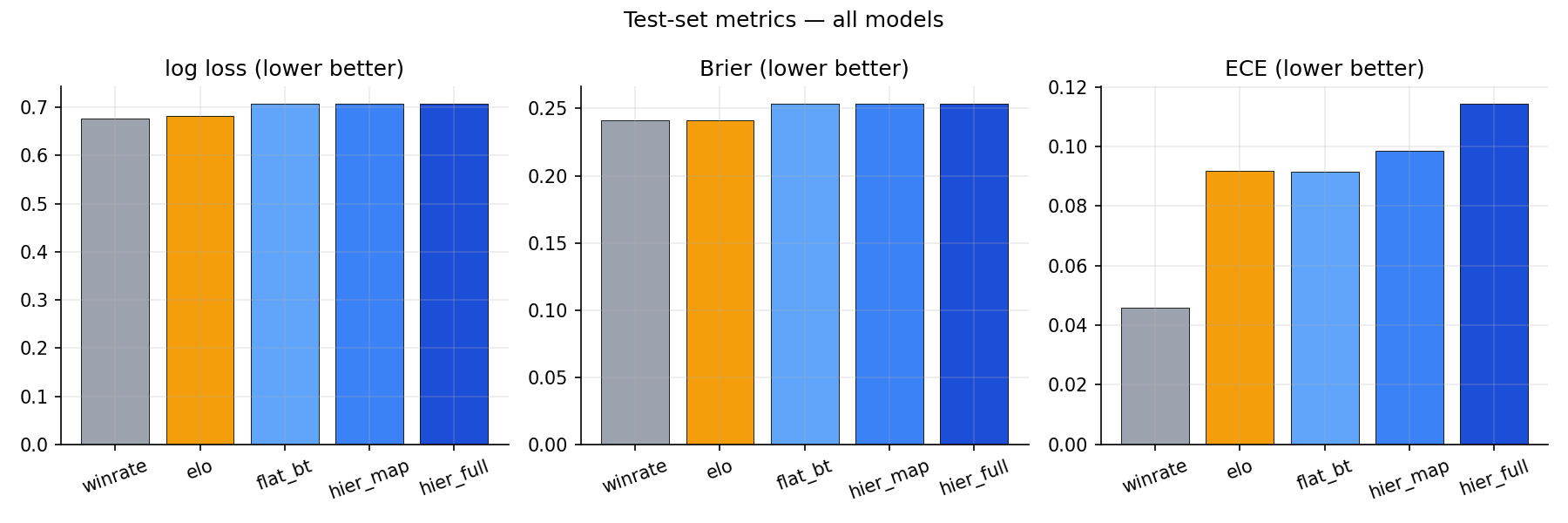
| Model | log loss | accuracy | Brier | ECE |
|---|---|---|---|---|
| Constant 0.5 | 0.693 | 50.0% | 0.250 | 0.000 |
| Win-rate | 0.676 | 60.4% | 0.242 | 0.046 |
| Elo (K=48) | 0.681 | 58.5% | 0.242 | 0.092 |
Elo barely beats win-rate on Brier, loses on log loss and ECE. The test slice is dense within-region late-season play where partner teams have already met repeatedly — cumulative win rate is highly informative. This is the bar to beat.
Phase 2 — Flat Bayesian Bradley–Terry
sigma_team ~ HalfNormal(1)
beta       ~ HalfNormal(1)
skill_t    ~ Normal(0, sigma_team)
P(A beats B) = sigmoid(beta * (skill_a - skill_b))
Fit with NumPyro NUTS, 1000 warmup + 1000 samples × 2 chains. R-hat max = 1.005; ESS min = 583; 0 divergences.
Test metrics: log loss 0.708, accuracy 58.5%, ECE 0.092. Slightly worse than Elo on the headline test slice, as expected — the value of this phase is plumbing. The model identifies FNATIC, Cloud9, LOUD, DRX, NRG, NaVi as the top-skill teams (skill posterior means 1.65 / 1.52 / 1.40 / 1.07 / 0.85 / 0.80 in logits), matching VCT 2023 standings.
Phase 3 — + Map hierarchy
Per-team, per-map effects with team-level partial pooling:
tau_map_global ~ HalfNormal(0.25)
tau_team_t     ~ HalfNormal(tau_map_global)
map_raw[t,m]   ~ Normal(0, 1)
map_effect[t,m] = tau_team_t * map_raw[t,m]
Teams with many observations on a map get well-pinned posteriors; teams with few get shrunk toward zero. R-hat max = 1.010; ESS min = 143; 0 divergences.
Headline test metrics: log loss 0.706 — basically tied with flat BT on within-region playoffs, and basically tied (0.6001 vs 0.6019) on the cross-regional held-out. The honest reading: the map hierarchy adds almost nothing above flat BT in this dataset. Per-team-per-map cells average ~16 maps each (502 maps / 30 teams × 9 maps), not enough to identify team-specific map effects above the shrinkage prior. With round-level outcomes (~25× the observations) or another season of data, this is the layer that would start to pull weight.
Phase 4 — + Region + time hierarchy
Two additional layers.
Regional pooling. Team skills draw from regional distributions:
sigma_region ~ HalfNormal(0.7)
mu_region[r] ~ Normal(0, 0.5)
skill_t      ~ Normal(mu_region[home_region(t)], sigma_region)
The 86 cross-regional matches at LOCK//IN provide the leverage to identify the regional means.
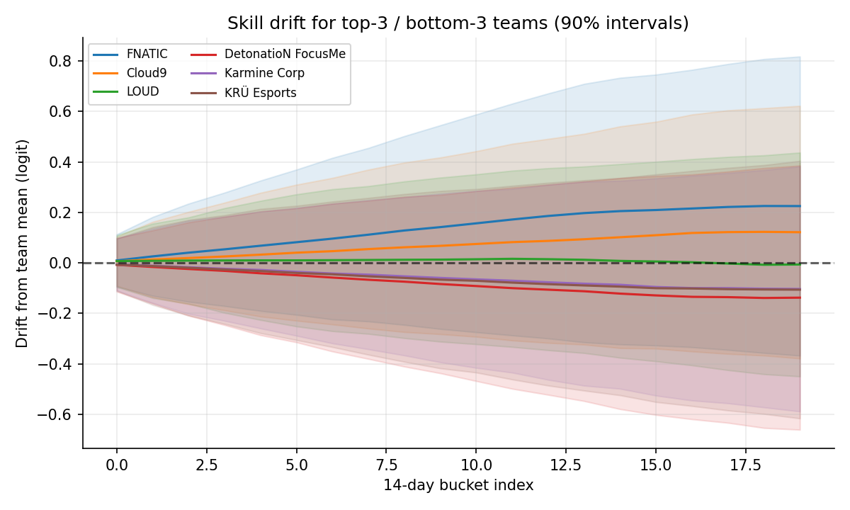
Time drift. A per-team random walk over 14-day buckets:
sigma_drift   ~ HalfNormal(0.06)
delta_raw[t,k] ~ Normal(0, 1)
drift[t,k]    = cumsum_k( sigma_drift * delta_raw[t, :k+1] )
Skill at any point = skill_t + drift[t, k]. For test prediction, drift is capped at the last training-period bucket — past that, the random walk is just adding variance from the prior without signal. R-hat max = 1.008; ESS min = 277; 0 divergences.
Posterior over regional means (logit-skill):
| Region | mean | 5% – 95% interval |
|---|---|---|
| Americas | +0.28 | [−0.35, +0.89] |
| EMEA | −0.02 | [−0.63, +0.59] |
| Pacific | −0.24 | [−0.88, +0.41] |
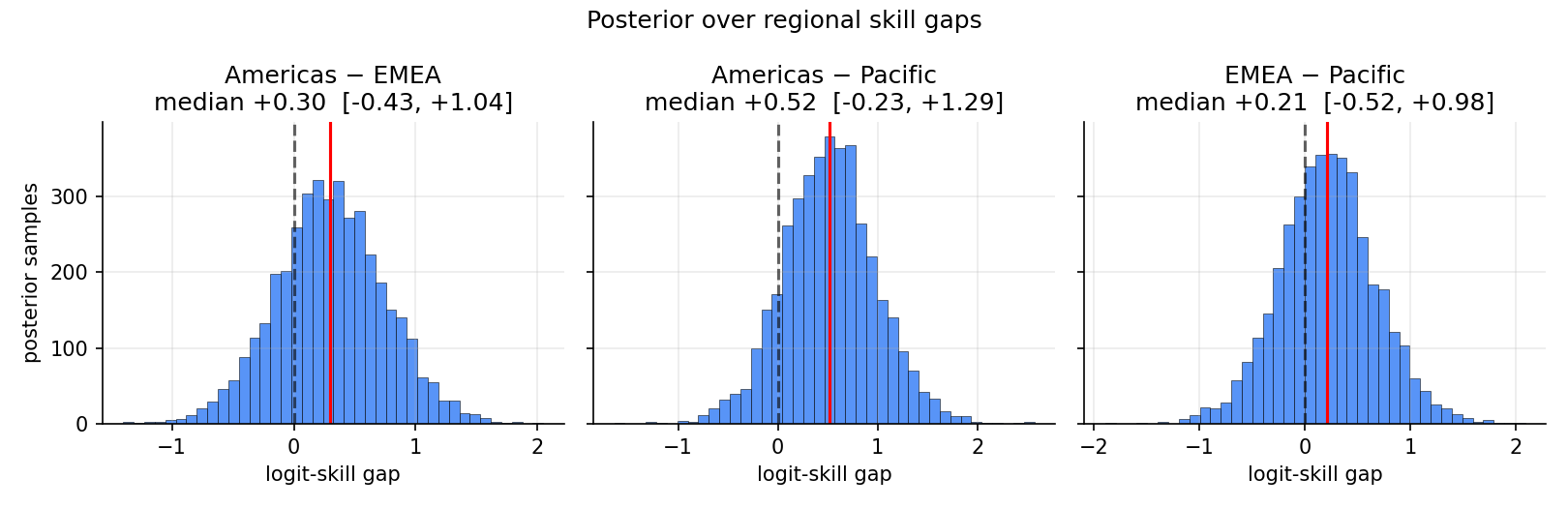
Posterior over pairwise gaps:
| Gap | median | 5% – 95% | P(a > b) |
|---|---|---|---|
| Americas − Pacific | +0.52 | [−0.23, +1.29] | 0.87 |
| Americas − EMEA | +0.30 | [−0.43, +1.04] | 0.76 |
| EMEA − Pacific | +0.22 | [−0.52, +0.98] | 0.69 |
Americas comes out ahead in this window — driven by LOUD, Cloud9, NRG, EG performances at LOCK//IN São Paulo. The credible intervals are wide because each pair is identified by ~30 cross-regional matches; the model is honest about how thin that signal is. Elo has no analog for any of these statements.
Phase 5 — Validation, calibration, ablation
Held-out cross-regional evaluation
The targeted test: hide every cross-regional match from training, refit each Bayesian model on within-region rows only, then predict the cross-regional matches.
| Model | log loss | Δ vs Elo | bootstrap 95% CI on Δ | accuracy | ECE |
|---|---|---|---|---|---|
| Win-rate | 0.6459 | +0.006 | — | 62.8% | 0.103 |
| Elo (K=48) | 0.6399 | — | — | 64.0% | 0.092 |
| Flat BT | 0.6019 | −0.038 | [−0.034, +0.106] | 66.3% | 0.069 |
| + Map | 0.6001 | −0.040 | [−0.031, +0.108] | 65.1% | 0.088 |
| + Region + Time | 0.5999 | −0.040 | [−0.019, +0.098] | 65.1% | 0.060 |
A few honest things:
- The improvement is suggestive, not significant at 95%. All three Bayesian models’ CIs cross zero (the full hierarchy’s lower bound is −0.019). Reproducing on a panel through Masters Tokyo + Champions LA — which roughly triples the cross-regional signal — is the natural way to push the CI clear of zero.
- Almost all of the improvement comes from the BT structure itself. Going flat BT → +Map → +Region+Time, the mean log-loss gap vs Elo barely moves (0.038 → 0.040 → 0.040). The +Map layer is a wash; the +Region+Time layer mainly improves calibration (ECE 0.069 → 0.060) rather than headline log loss. Why flat BT alone beats Elo on cross-regional: Bayesian skill estimates pool across the full set of within-region matches each team played, and the posterior-predictive average naturally regularises confidence; Elo’s online updates have no analog to either.
- Anchoring 0.040 in concrete terms. The Bayesian model assigns the actual winner an average of 57.1% probability (Elo: 53.5%, win-rate: 52.9%) — about 4 percentage points more probability mass on what really happened. On calls where the model is ≥70% confident, the full hierarchy lands them at 78.3% empirical across 23 calls; Elo only makes four such confident calls (so it dodges the test, basically).
- Even the win-rate baseline gets within 0.006 log-loss of Elo on this slice — there isn’t enough cross-regional repetition to make Elo’s online updating shine.
Headline test (within-region playoffs)
| Model | log loss | accuracy | ECE |
|---|---|---|---|
| Constant 0.5 | 0.693 | 50.0% | 0.000 |
| Win-rate | 0.676 | 60.4% | 0.046 |
| Elo (K=48) | 0.681 | 58.5% | 0.092 |
| Flat BT | 0.708 | 58.5% | 0.092 |
| + Map | 0.706 | 58.5% | 0.099 |
| + Region + Time | 0.708 | 58.5% | 0.115 |
Win-rate wins this slice — but not because it’s a generally superior model. By late-May playoffs, partner-league teams have played each other 20+ times, so cumulative head-to-head data is maximally informative; there isn’t much marginal signal left for hierarchical structure to extract. The contrast with the cross-regional slice — where teams meet once or twice and structure is the only thing that lets you generalize — is the slice-dependence story this writeup is built around. Model complexity should be paid for by what it identifies, and the data identifies different things on different slices.
Calibration
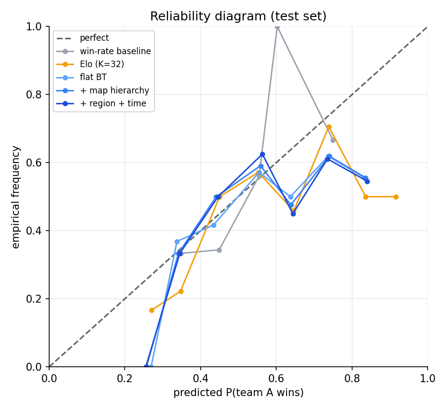
The reliability diagram shows what the ECE numbers compress: the win-rate baseline stays close to the diagonal because it never strays from 0.5 by much, while Elo and the Bayesian models get over-confident in both tails on the within-region slice.
Skill uncertainty vs data
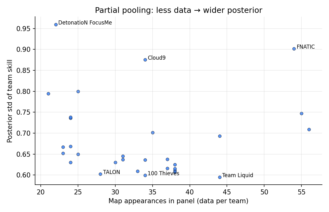
Posterior std of team skill drops as the team accumulates appearances. This is partial pooling on display: a team with five maps gets a posterior anchored by its regional prior; a team with seventy maps gets a tightly-pinned, data-driven estimate. Elo has no analog — every team’s rating has the same nominal certainty.
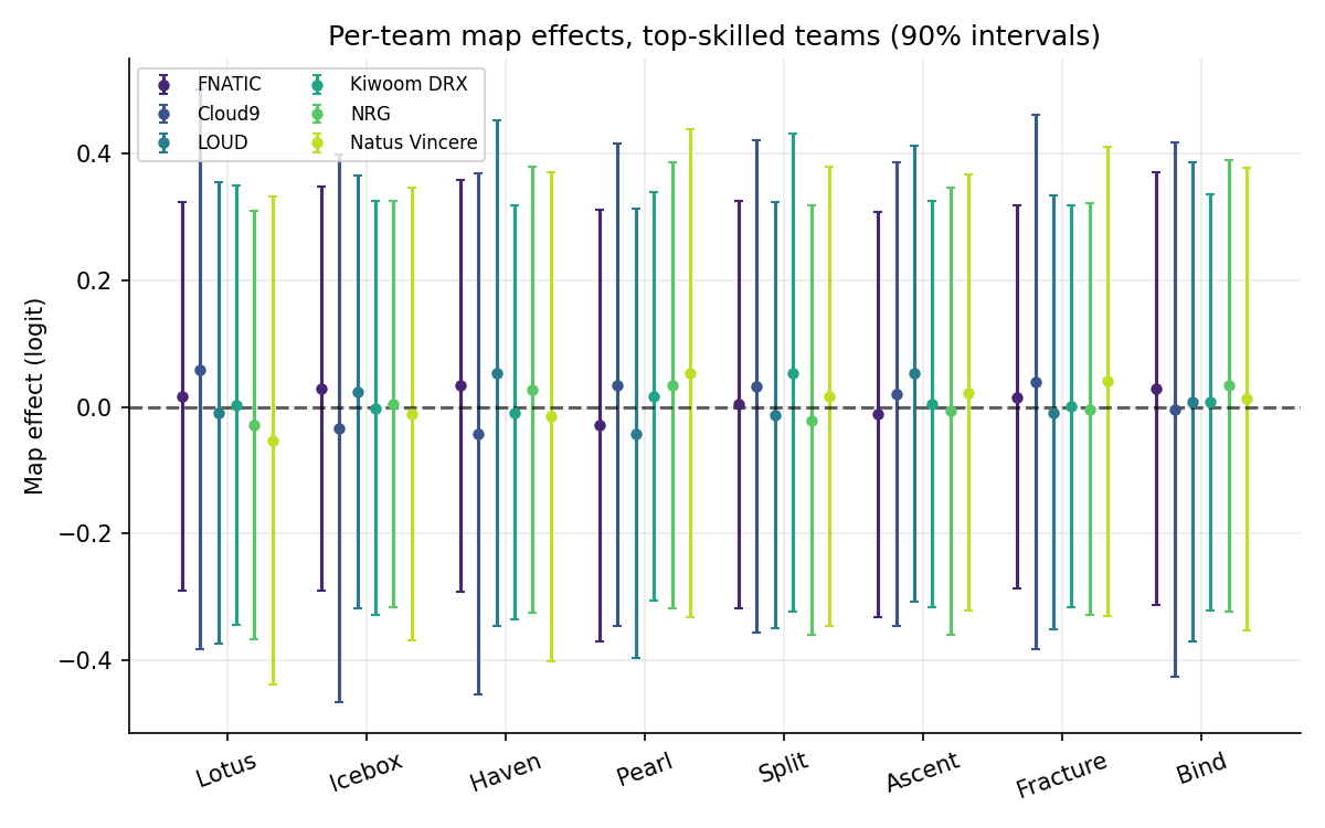
Top / bottom 12
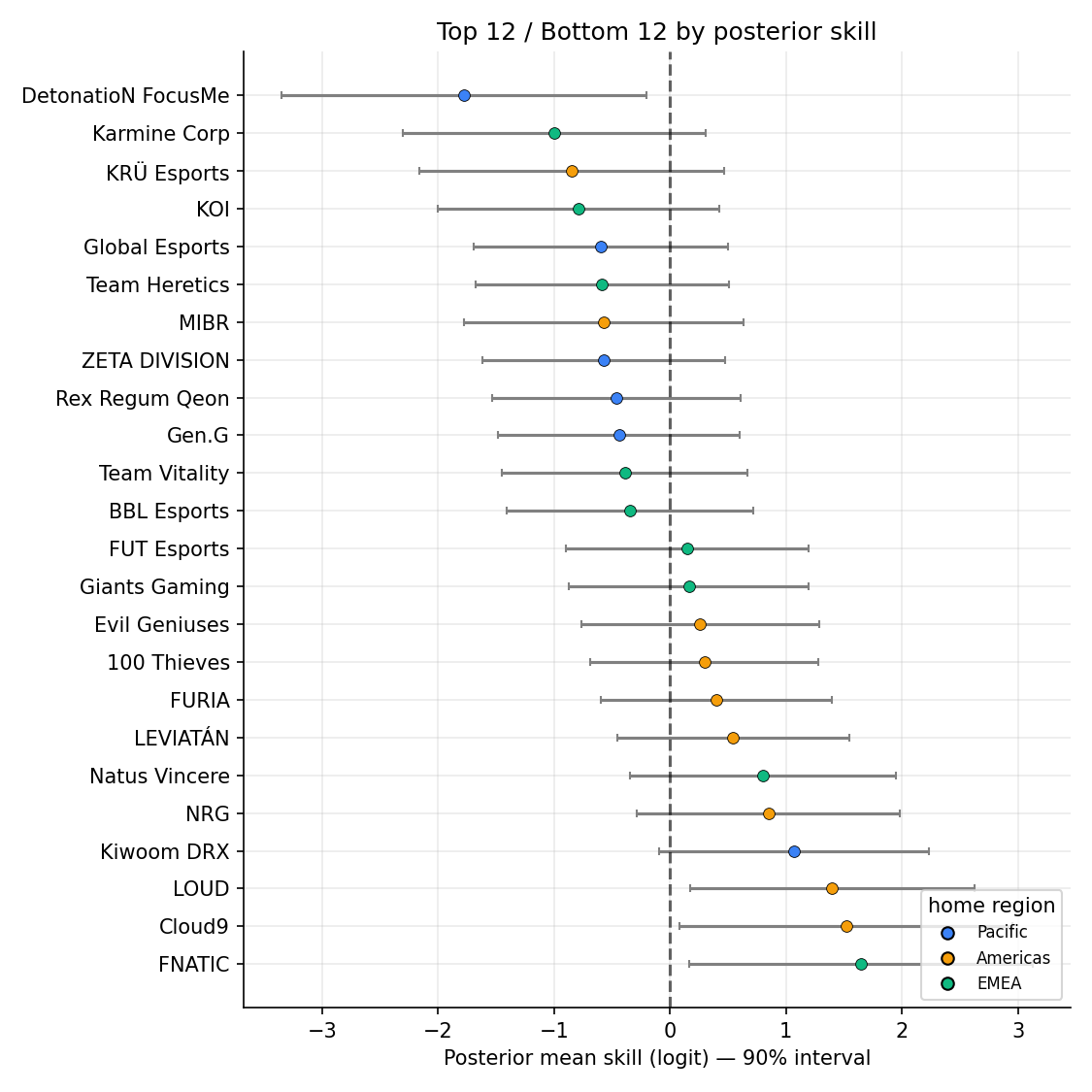
90% credible intervals for the highest- and lowest-skill teams. Spread within the top group is real (FNATIC and Cloud9 above LOUD with high probability); spread within the bottom group is mostly prior pull, since several have very thin records.
Ablation
What this leaves out
- No round-level data. Modeling at the round level (~25× more observations, plus side effects) is the natural next step but takes substantially more compute.
- No roster tracking. Roster changes are absorbed implicitly through the drift term. Explicit step changes at known roster moves would do better near transition dates but adds parameter-count and identifiability headaches.
- Short panel. The 9-month window predates Masters Tokyo (June 2023) and Champions Los Angeles (August 2023), the two events where the regional hierarchy is most stress-tested.
- 30-team set is the VCT 2023 partner cohort + a few Champions 2022 teams. Tier-2 / Challengers play is dropped to keep regional comparisons clean.
- No agent / map-pool composition. The Chamber project shows agent picks shift skill at the margin. A stretch goal is patch-aware ratings combining the two projects.
What I’d do next
- Expand the panel forward through Champions 2023. That would add ~150 cross-regional matches and turn the cross-regional held-out into the primary test slice rather than a targeted one.
- Round-level model with side effects.
P(round won by attacker) = sigmoid(skill_atk + map_atk_eff − skill_def − map_def_eff + side_advantage[map]). Captures the most important within-map structural feature. - Player ratings as a second hierarchy. Each team’s skill = sum of player skill + team chemistry. Identifiable when rosters change (which they do, multiple times per year).
- Variational inference for the round-level extension. At ~500 maps, NUTS finishes in seconds and SVI buys nothing. The case for SVI shows up at round-level (12k+ observations × side effects × per-map structure), where MCMC moves from seconds to minutes per refit.
Reproduce
pip install -r requirements.txt
python -m src.data
python -m scripts.run_baselines
python -m scripts.run_flat_bt
python -m scripts.run_hier_map
python -m scripts.run_hier_full
python -m scripts.run_held_out_xreg
python -m scripts.run_bootstrap
python -m scripts.run_ablation
Total runtime end-to-end: ~90 seconds on a 2024 laptop CPU.